A Brief High Analysis of Shell Eco-marathon Telemetry Data

Shell Eco-marathon is an annual event sponsored by Shell where students all around the world competing building most energy-efficient vehicles. During each race attempt, participants vehicles are equipped with electronics instrument to monitor vehicles data.

After each successful attempt, Shell eco-marathon technical team provided the telemetry data to participant to be analyze for strategy improvement for next attempt.

In this post I am going to analyze telemetry data of Team Horas USU urban diesel car, which provided by Shell Eco-marathon technical team, to get an insights of Team Horas Urban car performance with the aim to optimize urban car results in future events.

At the end of the post I'll also iteratively estimate the performance of the vehicles with different specification such as weight by using this telemetry data.

Data Format

Technical team of Shell Eco-marathon provided telemetry data of particpant attempt in form of csv files. This helps team to analyze telemetry data quickly by using programming languages such as python to process and plot data.

This is crucial beacuse it enable team to make a high analysis of each attempt to help improve their next attempt in very short amount of time.

There are multiple vehicle parameter that monitored by Shell Eco-marathon, such as:

1. Vehicle speed
2. Fuel instantaneous flow
3. GPS coordinates
4. Electrical energy (voltage, current).

Coast and Burn

Most team in Shell Eco-marathon using a coast and burn drive cycle strategy to minimize its fuel/energy consumption.

Coast and burn strategy is an eco driving style where a vehicle start an engine and accelerate to certain speed (burning period) then turn the engine off. Vehicle starts gliding (coasting period) even after then engine off, and then decelerate to lower speed to the point where the engine need to start again, and process is repeated.

This is the reason teams try to minimize vehicle mechanical friction, and design an aerodynamics shape body to help reduce de-acceleration cause by other resistances force acting on the car when the car is moving.

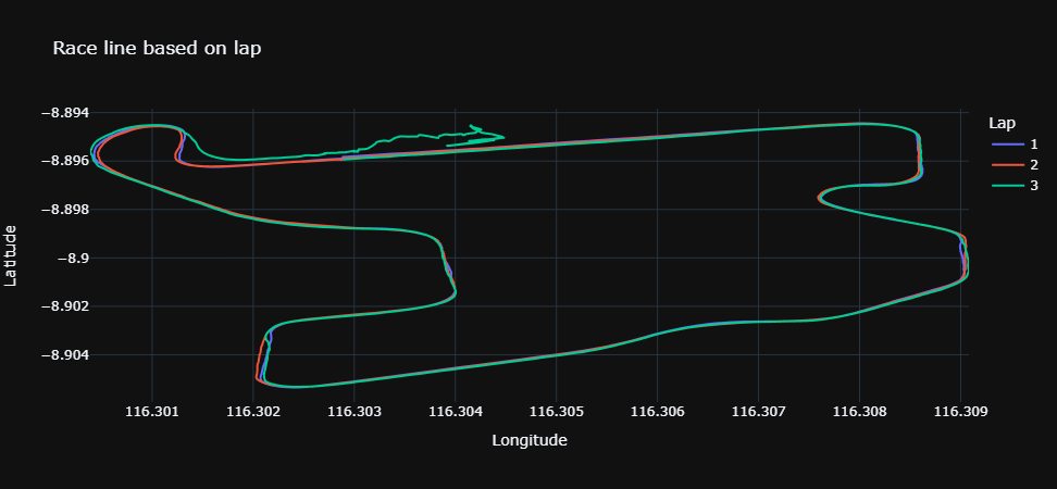
You can see the coast and burn pattern on the track in this figure below:

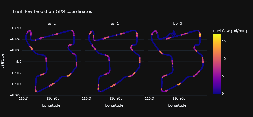
Figure 1. Fuel flow vs vehicle Position

Because this driving cycle, choosing when to start the engine and turn it off is crucial. For a car powered by internal combustion engine, speed is an important aspect to maximize fuel efficiency.

Internal combustion engine has its own characteristics where certain range of rpm capable of producing the most power while consume least amount of fuel. This fuel consumption and power relation is expressed with this equation.

sfc$\ =\frac{\dot{m_f}\ \times\ 10^{3}}{P}$

• - sfc = specific fuel consumption (g/kWh)
• - $\dot{m_f}$ = mass flow rate of fuel (kg/h)
• - P = Power (kW)

Here you can see an example of specific fuel consumption graph of an engine.

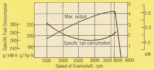
Figure 2. SFC Graph

Ideally team try to run the vehicle/engine on the lower part oh the sfc graph.

Lap Comparison

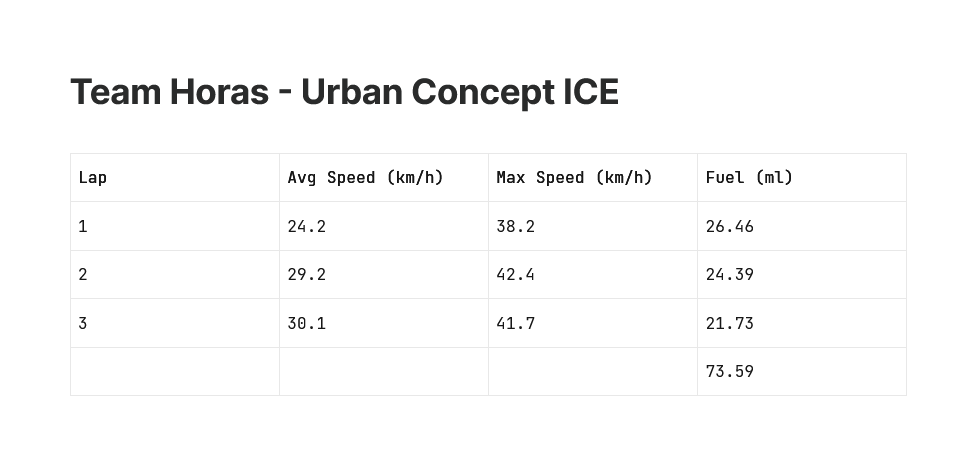
Figure 3. Lap comparison table

From the picture above you can see fuel efficiency increase as lap progress, with lap #1 with the highest amount of fuel being used, and lap #3 the least. If we can copy driving characteristic/style in lap #3 to other two laps, we could end up with end result 65.19 ml. That's mean around 11% fuel consumption improvement.

It is only logical to look what the driver did different on each lap to know what could possibly affect efficiency of fuel consumption. Easiest parameter to look at is speed of the vehicle.

Based on Figure 2 it seems Team Horas Urban car perform a better fuel efficiency when running on higher speed. But, lets take a detail look at car speed on each lap.

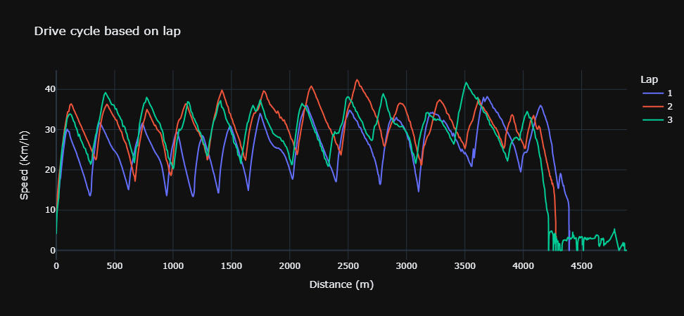
Figure 4. Speed vs Distance

From picture above we can see that lap #2 and #3 which has a better fuel efficiency than lap #1 as most of the time it reach higher top speed above 32 km/h and start the engine at higher speed around 20 km/h compare to lap #1 where it only start the engine around 15 km/h.

Beside speed, lap #3 was also perform better than the other laps becasue it has less burn spot (+-12) than the other two laps (+-13). We can tell number of burn period by looking at the engine state. Engine state indicated by certain electrical current (2 ampere for this car) and fuel flow. Sometime there might be a fuel flow in the flowmeter despite the engine wasn't actually running.

data["did_fuel_flow"] = np.where(data["lfm_instantflow"] > 0, 1, 0)
data["did_current_flow"] = np.where(data["jm3_current"] < 2000, 0, 1)
data["engine_state"] = data["did_current_flow"] * data['did_fuel_flow']

Here is engine state of the car on each lap:

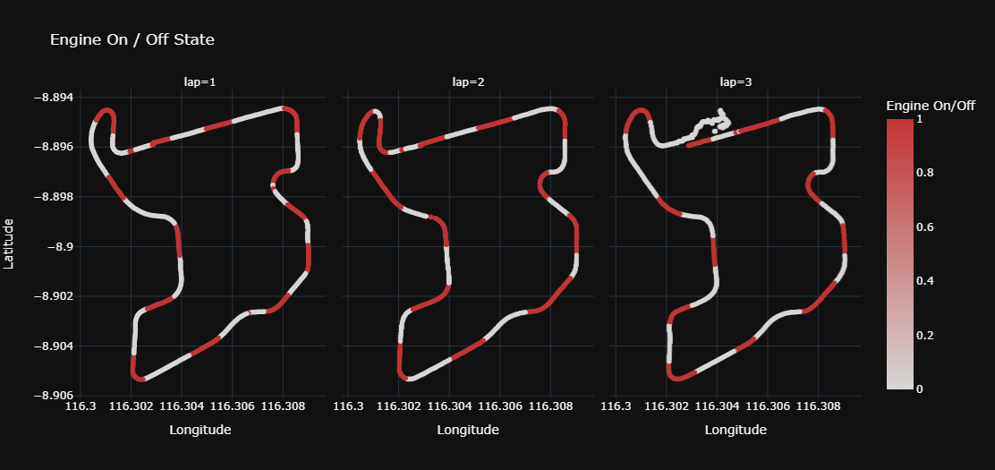
Figure 5. Engine On/Off State based on Lap

Reducing burn-coast period also mean less motor starter usage therefore less energy (electrical energy). Less motor starter usage is quite important for vehicle with high compression ratio engine such as diesel/ethanol fuel powered engine for it require more power to start/crank the engine.

Vehicle Dynamics Modelling

For 2024 season Team Horas newest generation release its new version of car. The car now using carbon fibre, replacing fiber glass for its body material and alumunium for the chassis. It reduced around +- 50 kg of weight. With this new car I want to estimate the efficiency improvement after weight reduction of the car using this telemetry data.

To be able estimating the newer car fuel consumption, first we need to know the sfc of the engine. Engine sfc can be derive by computing vehicle dynamics and the fuel instantaneous flow from telemetry data. Specific fuel consumption then can be plug to the newer car vehicle dynamics to calculate the amount of fuel needed to perform the same speed profile from the telemetry data.

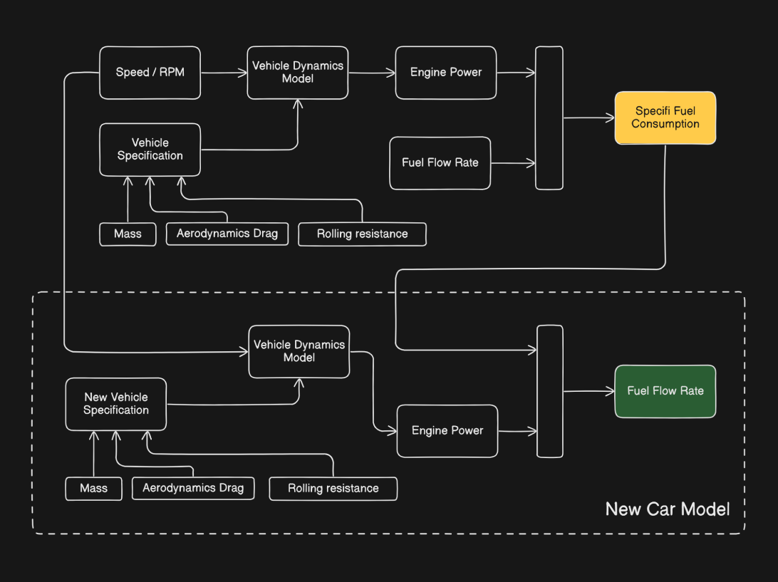
Figure 6. Fuel Consumption Model

Specific Fuel Consumption

Engine SFC can be calculated with this equation:

sfc$\ =\frac{\dot{m_f}\ \times\ 10^{3}}{P}$

• - sfc = specific fuel consumption (g/kWh)
• - $\dot{m_f}$ = mass flow rate of fuel (kg/h)
• - P = Power (kW)

Engine power can be derived from the tractive force of the car and its rpm. Here is how the car force can be derived:

$ma(t) = {F_{trac}(t)} - F_{res}(t)$

• - $F_{trac}(t)$ = Tractive Force (N)
• - $F_{res}(t)$ = Cumulative resistance forces (N)

There are at least 4 type of resistance force acting on a vehicle; Inertia force, drag force (Aerodynamics), rolling resistance force, and gradient force.

${F_{res}} = {F_{inertia}} + {F_{drag}} + {F_{rolling\_resistance}} + {F_{grad}}$

Or can be breakdown to:

${F_{res}} = {(ma)} + {(\frac{ρv^{2}{C_d}A}{2})} + ({C_{rr}}mg) + ({mg \times\sinα})$

• - m = Vehicle mass + Driver (kg)
• - a = Vehicle acceleration (${m/s^2}$)
• - g = Gravity (${m/s^2}$)
• - v = Velocity (m/s)
• - ρ = Air density (${kg/m^3}$)
• - $C_{d}$ = Coefficient of drag
• - A = Frontal area of car ($m^2$)
• - $C_{rr}$ = Rolling coefficient of tyre

Here is the free body diagram of vehicle dynamics:

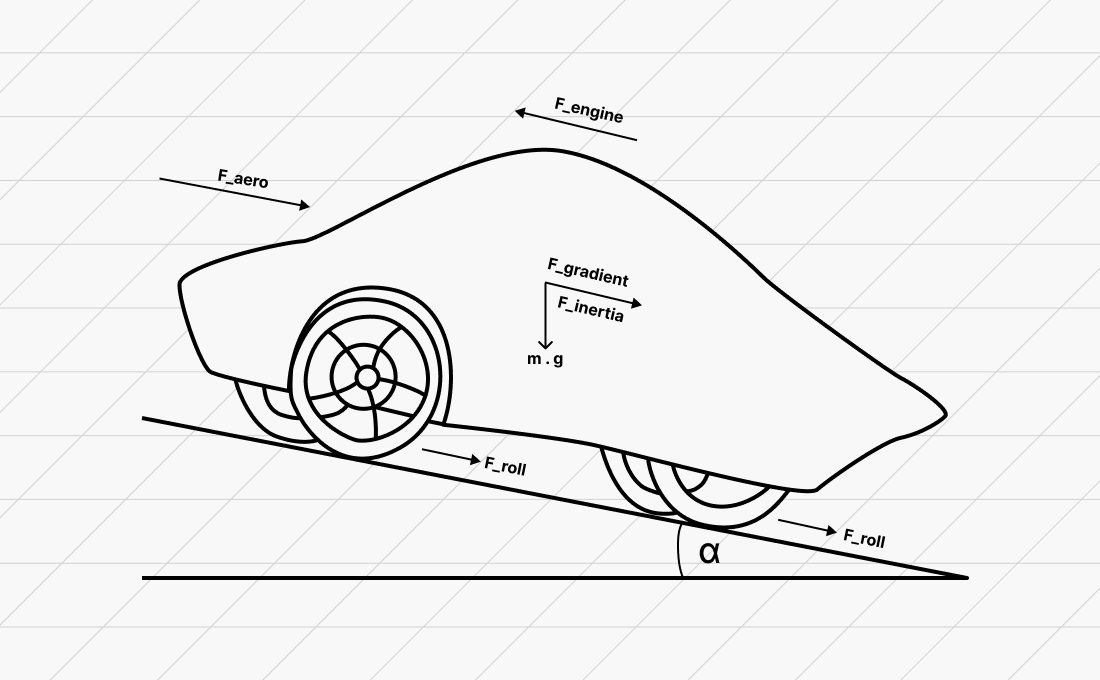
Figure 7. Vehicle Dynamics

We have all of the data needed except the α for the gradient force. The α is the difference in elevation of two given point in the track. I tried to get the elevation of the track using Google Maps elevation API by utilizing the gps coordinates from telemetry data.

import request
 
# API call for retrieving location elevation
def request_elevation(long, lat):
    url = "https://maps.googleapis.com/maps/api/elevation/json?locations=" + str(lat) + "%2C" + str(long) + "&key=YOUR_API_KEY"
 
    response = requests.get(url)
 
    if response.status_code == 200:
        json = response.json()
        elevation = json["results"][0]["elevation"]
        return elevation
 
    return float("NaN") ## Perform data cleaning later on
 
 
# Inserting the elevation data to the dataframe
data["elevation"] = request_elevation(data["gps_longitude"], data["gps_latitude"])
data["elevation"] = data["elevation"].ffill()

Based on the Google maps Elevation API here is how the elevation of Mandalika Circuit:

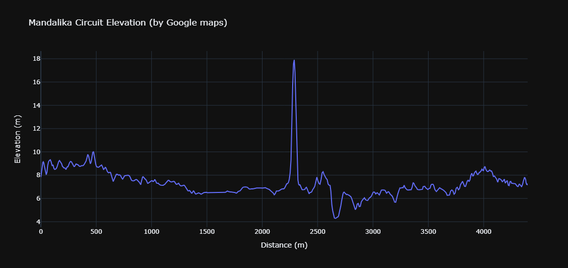
Figure 8. Track Elevation from Google Maps elevation API

I cross checked the accuracy of the elevation data with the driver, it seems that Google maps API is not that accurate (at least for Mandalika Circuit). So due to its limited data of track elevation, gradient force is assumed to be zero (α = 0) for this vehicle dynamics model.

After obtained all the model parameter, We can finally compute the model:

# Vehicle dynamics (Urban Diesel - Team Horas USU)
F_Grad = 0 ## Due to limited data of circuit elevation, it assumed to be 0
data["force_push"] = data["force_drag"] + data["force_inertia"] + F_RR + F_Grad
data["engine_torque"] = data["force_push"] * TYRE_RADIUS / GEAR_RATIO
data["engine_power"] = 2 * 3.14 * data["engine_torque"] * data["rpm"] / 60000
data["fuel_instantflow"] = data["sfc"] * data["engine_power"] / 60 / 0.85
data["fuel_instantflow"] = data['fuel_instantflow'].fillna(0)
data["fuel_in_ml"] = data['fuel_instantflow'] / 60
 
electricalEnergyToFuel = data["jm_power"].sum() / 0.25 / 0.75 / (0.7646 * 42900) # calculation derived from Shell Eco-marathon rules.
distances = 4300 * 3 # 4300 meter each lap, total 3 lap
cumulatedFuel = data["fuel_in_ml"].sum()
 
fuelEfficiency = distances / cumulatedFuel # km/l
energyEfficiency = distances / (cumulatedFuel + electricalEnergyToFuel) # km/l

This is an example of fuel consumption (actual and estimation) comparison before and after weight reduction.

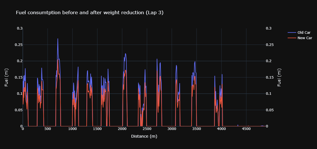
Figure 9. Fuel Consumtption before and after weight reduction (Lap 3)

Here is the final result of the calculation:

• - Distance: 12900 meters
• - Fuel consumption: 52.19 ml (73.59 ml for previous car)
• - Electrical energy consumption to fuel consumption (ml): 17.70 (Assumption: Same electrical energy usage)
• - Result (fuel only): 247 Km/l
• - Result (total energy): 184 Km/l

This mean by reducing weight of the car for 50 kg, team would be able to increase efficiency from 130 Km/l to 184 Km/l (43% improvement).

Final result could go much higher assuming an improvement in engine thermal efficiency, gear ratio variation, and better drive cycle. Car could also covered more distance during coast period after the weight reduction.